Chromatic Polynomials 01 - Introduction

Through this article and the next several articles, I’m going to share with you something called Chromatic Polynomials. It’s a form of math that is quite powerful in its most basic form, but I’ll show you how to make it even more so. I’ll show you how to apply chromatic polynomials to sudoku, logic puzzles, video poker, slot games, B-Sat problems, and more.

I first learned about chromatic polynomials from the paper “Counting complex disordered states by efficient pattern matching: chromatic polynomials and Potts partition functions”, by Marc Timme, Frank van Bussel, Denny Fliegner, and Sebastian Stolzenberg, published in the New Journal of Physics on February 4, 2009. This first article presents the basics of chromatic polynomials, as presented by Timme et al. In later articles, I’ll show you some expansions of the chromatic polynomial syntax to increase their capabilities, and some novel ways to use those capabilities.

Kronecker Deltas

Understanding chromatic polynomials starts with understanding Kronecker Deltas, named after the mathematician, Leopold Kronecker. A Kronecker Delta is a function that compares two values and returns a 1 if they are equal and a 0 if they are not. It is typically defined as:

The Kronecker Delta is much like the ternary operator in the C programming language: i == j ? 1 : 0. It could also be represented in C as (i == j).

Graph Coloring

The term “chromatic polynomial” refers to a polynomial solution to a graph coloring problem. The problem is presented as a graph consisting of vertices connected by edges, such as this:

Graph 1 has four vertices, σ₁ - σ₄, and two edges, σ₁σ₂ and σ₁σ₃. The question posed is:

Given Q unique colors, how many ways can we assign a color to each vertex such that no two vertices connected by a line have the same color?

We can assign any one of the Q colors to σ₁. Then, we can assign σ₂ and σ₃ any color except the one chosen for σ₁, or Q-1 colors each. And we can assign σ₄ any one of the Q colors, since it is not connected to any other vertex by an edge and is therefore has no constraints on the color selected. Thus, the number of solutions to this coloring problem is Q*Q*(Q-1)*(Q-1) = Q²(Q-1)². This is the chromatic polynomial for Graph 1.

And this is the meaning of “chromatic polynomial”: Q²(Q-1)² is the polynomial that solves this chromatic (coloring) problem. From here on, I’ll be using the abbreviation “CP” for chromatic polynomial.

Of course, once the polynomial is known, Q can be replaced with a concrete value. Given 2 colors (Q = 2), there are 2²*(2 - 1)² = 4 ways to color graph 1. Given 3 colors (Q = 3) there are 3²*(3 - 1)² = 36 ways to color graph 1.

This example was easy to work out by hand. For more complex cases we need the methods taught by Timme et al. It starts with an expression that represents the graph:

For each vertex, we specify a summation over all of its possible values. For each edge, there is a term containing a Kronecker delta that excludes matching values for the two vertices connected by that edge. For the edge σ₁σ₂ we specify the term (1- δ_σ1σ2). For the edge σ₁σ₃ we specify the term (1 - δ_σ1σ3). The rules for summation are as follows:

Rule 1: A summation for a vertex in a Kronecker delta reduces that Kronecker delta to 1.

The easiest way to understand this is to say, “We don’t yet know the value of σ₂, but we know it must have a single value. Therefore, there is only one way to assign a value to σ₁ such that it matches σ₂.”

To be a bit more thorough, we can see that through the summation, σ₁ takes every possible value from 1 to Q:

Of those Q values, only one can match σ₂:

Rule 2: Any term that does not contain the vertex being summed over is multiplied by Q:

This is because the summation expands to Q copies of the term, unmodified by the vertex being summed over. This also implies that:

And:

And any combination thereof:

Combining this with Rule 1 gives us cases like this:

And:

Rule 1 and Rule 2 together show us that:

That is, if there are Q possible values for σ₁ and σ₂, then there are Q ways that σ₁ = σ₂, as shown by this chart:

δσ1σ2 =	σ1 = 1	σ1 = 2	σ1 = 3	. . .	σ1 = Q
σ2 = 1	1	0	0	. . .	0
σ2 = 2	0	1	0	. . .	0
σ2 = 3	0	0	1	. . .	0
. . .	. . .	. . .	. . .	. . .	. . .
σ2 = Q	0	0	0	. . .	1

Rule 3: When two Kronecker deltas specify that one vertex’s color is equal to two other vertices’ colors, then those two other vertices colors must be equal:

This is basically a transitive property of Kronecker deltas - if σ₁ = σ₂ and σ₁ = σ₃, then σ₂= σ₃. Here’s a more extreme case:

In general:

When starting out with CPs, it’s best to explicitly include all of these Kronecker deltas. It is cumbersome, but necessary to ensure that conditions are not accidentally dropped while summing. This is because summing over a specific vertex eliminates every instance of that vertex:

Later, I will show a more elegant way of handling this case.

Graph 1, using summations

We are now ready to find the CP for Graph 1 using summations. To represent the edge connecting σ₁ and σ₂ we include the term (1- δ_σ1σ2). the edge connecting σ₁ and σ₃ we include the term (1- δ_σ1σ3).

One more rule

Before summing over a vertex, all terms containing that vertex must be expanded. To sum over σ₁, we must expand the polynomial to:

Per Rule 3, the last term must be expanded to include all combinations:

Summing over σ₁ yields:

Summing over σ₂ yields:

Summing over σ₃ yields:

Summing over σ₄ yields:

This is identical to the solution worked out by hand above:

Order affects expansion

Note that if we choose to sum over σ₂ first, we do not need to expand the terms, since only one of the terms contains σ₂:

Summing over σ₂ first yields:

When summing over σ₁, we can leave the (Q - 1) term alone and sum (1 - δ_σ1σ3):

Summing over σ₃ and σ₄ will produce the same final solution as the above: Q²(Q - 1)².

Exercises

These exercises are provided for you to test your understanding of CPs. The solutions are provided below. Transcribe each of these graphs into a summation formula, then sum over each vertex to derive the CP.

1a	1b	1c
1d	1e	1f
1g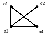	1h	1i

Solutions to Exercises

1a

Since there are no edges to this graph, there are no constraints placed on any of the vertices:

1b

Since only σ1 and σ3 are connected by an edge, there is only one constraint:

1c

1d

1e

1f

1g

1h

1i

Previous Post:

www.solutionslookingforproblems.com

Searching for a 3x3 magic square of Squares

IntroductionThe question of whether it is possible to create a 3x3 magic square of squares is an unsolved problem in mathematics. There have been many attempts at finding a solution, resulting in many “near misses” - solutions that meet some of the requirements but not all of them. There is an excellent summary of research and attempts at solutions at http://www.multimagie.com/English/SquaresOfSquaresSearch.htm.Here, I will present a purely algebraic approach to a 3x3 magic square of squares, an

Next Post:

www.solutionslookingforproblems.com

Chromatic Polynomials 02 - Almost a Language of Logic

In the previous article, we saw that each edge in a graph represents a condition. That condition is transcribed into a term to be multiplied with other terms. The result of the summation is the number of ways that all the specified conditions can be met.Logical NOTIn an unsummed CP, a 1 represents all the unconstrained possibilities. As shown in exercise 1a, from the previous article:The term (1 - δσ1σ2) represents “All the unconstrained ways, minus the ways that σ1 is equal to σ2”. This shows u