Chromatic Polynomials 03 – Expanding the Capabilities

This article outlines modifications that I came up with to expand Chromatic Polynomials into a fully-capable language of logic.

Constants instead of variables

The traditional Kronecker Delta compares two variables, e.g. δ_ij compares i and j. We could just as easily replace one of those variables with a constant value:

This changes the rules for summation a little bit:

That is, of all the values that i can take, only one will be 3. This allows us to specify that a vertex must match a specific value, e.g. δ_σ1,3, or that a vertex must not match a specific value, (1-δ_σ1,3).

Note that this has some implications for multiplying Kronecker Deltas:

It is also safe to add Kronecker Deltas when constant values ensure that terms are mutually exclusive:

Kronecker deltas with multiple constants

Knowing that different constant values are mutually exclusive, we can introduce a bit of syntactic sugar to combine Kronecker deltas with multiple constants into one:

I chose a set-like notation for the constants: {3,4}. This helps separate the constants from the variable. I also sometimes specify ranges with {0-5,7,12,20-24}. Note that ‘-‘ inside a Kronecker delta does not mean subtraction; it means a range of values. “20-24” means “20, 21, 22, 23, 24”.

Since each constant represents a unique value that the variable can take, summing over a Kronecker delta with a set of constants produces the size of the set:

Multiplying two Kronecker deltas with the same variable and two different sets of constants results in the intersection of the two sets of constants:

If the intersection is the empty set, then the product is 0:

And finally, the transitive property still applies:

And

But watch out! Kronecker deltas can specify two variables that each must match the same set of constants, but this does not imply any relationship between those two variables:

More than two vertices per Kronecker delta

In the introduction to Chromatic Polynomials, I showed this monstrosity:

It’s necessary to know all the equalities implied by a chain of Kronecker deltas like this, but writing this out is very cumbersome. Instead, we can apply a little more syntactic sugar and replace the entire chain with a single “Extended Kronecker delta”:

In my Chromatic Polynomial engine, since I’m a lazy typist, I also added this syntax:

A Kronecker delta with more than two vertices no longer represents the edge of a graph, but the connection could be represented with a hypergraph. The Kronecker delta’s definition is extended to this:

The summation for an Extended Kronecker delta is:

And

Multiplying EKDs

Extended Kronecker deltas (EKDs) that are multiplied together can be combined if they have at least one vertex in common or if they both share the same single constant. The set of variables in the product EKD is the union of the factor EKDs’ variables. The set of constants in the product EKD is the intersection of the factor EKDs’ constants.

Multiplying EKDs Example 1 – EKDs with common vertices:

These two multiplied EKDs can be combined into a single EDK, since they share the vertex σ₁. The vertices will be the union of the two EKDs’ vertices:

The constants will be the intersection of the two EKDs’ constants:

The final result is:

Multiplying EKDs Example 2 – EKDs with a common single constant:

Since each EKD states that all vertices must equal the same constant, these can be combined. The vertices will be the union of the two EKDs’ vertices. The constant will remain:

Note that when two multiplied EKDs have the same single constant, they do not need to have any vertices in common.

Adding EKDs

EKDs that are added together can be combined if they have the same set of vertices and mutually exclusive sets of constants. The combined EKD’s set of constants is the union of those EKDs added together.

Adding EKDs, Example:

This example shows two EKDs with the same variables and non-intersecting sets of constants:

This works because the size of the union of two non-intersecting sets is the sum of the sizes of the two sets:

For EKDs this means that:

EKDs that cannot be added:

These cannot be added because the two EKDs do not have the same set of variables:

These cannot be added because the two EKDs have overlapping sets of constants:

Summation Shorthand

Because every CP exercise involves summation over all the vertices, I find it convenient to apply the same range shorthand to summations that I apply to lists of vertices and constants:

Miscellany

Here are a few miscellaneous extensions to CPs.

Summing over Concrete Ranges

Rather than summing each vertex to a variable, e.g. Q, we can sum over a concrete value:

The rules for summation are the same, except that we replace Q with 5 in the summation. This is useful if we want an answer for a specific range and not a generalized solution. In many cases, it is more efficient as it allows terms to be reduced more quickly (e.g. Q + Q² cannot be reduced, but 5 + 25 can):

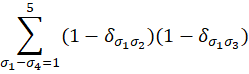
= 400

Different Ranges

We may want to compare two vertices, but sum them over different ranges. We may be tempted to write something like this:

This is a badly-formed expression. If it produces a correct answer, it is purely by accident.

This expression specifies that δ_σ1, must be in the range [1-3], δ_σ2 must be in the range [1-5], but they cannot match. Summing this by the given rules will produce 10 if we sum over δ_σ1 first and 12 if we sum over δ_σ2 first.

Summing over δ_σ1 first yields:

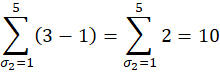
Summing over δ_σ2 first yields:

To apply a specific range to a vertex, use the extended Kronecker Delta with constants to specify σ₁’s range:

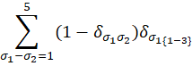
15 - 3

12

NOTE: It is possible to sum vertices over different ranges as long as those vertices are not present in the same EKD and will never be compared to one another by any expansion of terms:

120

Since the terms don’t interact, we can highlight the separation like this:

This shows that there are two separate sets of vertices which do not interact with one another. I also find that the summation shorthand helps reinforce the concept that vertices in the same EKD must be summed over the same range:

Summing to Probabilities

It is also possible to alter the summation rules to generate probabilities:

For me, this is a frivolous exercise. If I want a probability, I would rather sum over discrete values, and then divide by the total number of possibilities. For n vertices summed from 1 to Q, the total number of possibilities is Qⁿ:

Assigning a constant value to a vertex

In some cases, we may be given a partial solution, e.g. σ₁ = 3. Applying this is as easy as replacing σ₁ with 3 in the original expression and removing the summation for that vertex. This provides an opportunity to reduce some terms prior to summing:

Note that we can accomplish the same effect by multiplying the entire expression by an EKD which limits the variable to the assigned constant:

This concludes the expansion of the capabilities of Chromatic Polynomials. All later articles will be dedicated to examples of what we can do with this Language of Logic.

Previous Post:

www.solutionslookingforproblems.com

Chromatic Polynomials 02 - Almost a Language of Logic

In the previous article, we saw that each edge in a graph represents a condition. That condition is transcribed into a term to be multiplied with other terms. The result of the summation is the number of ways that all the specified conditions can be met.Logical NOTIn an unsummed CP, a 1 represents all the unconstrained possibilities. As shown in exercise 1a, from the previous article:The term (1 - δσ1σ2) represents “All the unconstrained ways, minus the ways that σ1 is equal to σ2”. This shows u

Next Post:

www.solutionslookingforproblems.com

Chromatic Polynomials 04 – My CP Symbolic Math Engine

I debated whether I should write anything about my CP application and came to realize that I need this article to provide context for formulas and scripts in later articles. You might see some large CPs later and think “There’s no way he did this by hand.” … and you would be right. I love studying CPs, but I’m too lazy and too impatient to do it all on paper. I wrote my own symbolic math engine to process Chromatic Polynomials for a few reasons:1)    I didn’t expect an existing math application